The Implications of Declining Wealth-to-GDP
Why more on this topic?
About ten days ago, we published the October 2022 Absolute Return Letter under the title The Rise of Wealth-to-GDP … and the Long Road to Normalisation. We received an unusually high number of replies to that letter, mostly from readers who had one or two genuine questions but also from readers who disagree with my conclusions.
Whether you buy into the storyline or not, I hope I can convince you to spend 20 minutes to read what is to follow; why wealth cannot continue to grow faster than the underlying economy, and what the investment implications of that are.
I am perfectly aware that there is an element of repetitiveness in this research paper when compared to the October Absolute Return Letter; however, in hindsight, I don’t think the October letter provided a good enough explanation as to why it is that wealth cannot outgrow GDP longer term.
Furthermore, as I have pointed out before, the UK regulator no longer allows us to offer investment advice in a freely distributed publication like the Absolute Return Letter. As I would like to share with you my thoughts on the investment implications of declining wealth-to-GDP, it became an easy decision.
A recap of the facts
The October Absolute Return Letter concluded that:
1. wealth cannot grow faster than GDP in the long run;
2. every time wealth-to-GDP deviates from its long-term mean value, it reverts to the mean;
3. wealth consists predominantly of private property, retirement savings, investments and business interests;
4. wealth-to-GDP is not the same in every country, yet it is long-term stable everywhere in the capitalist world;
5. wealth-to-GDP varies from country to country because capital efficiency (i.e. how much capital it takes to produce $1 of output) is not the same everywhere.
In the following, I will not go into an in-depth discussion on any of these points but assume you have already read the October letter and are familiar with the thinking behind it. If you think the October letter doesn’t answer all your questions, I suggest you read some of the other papers I have written on the topic, for example the megatrend paper on debt super cycles from September 2019.
The underlying logic
If I am prepared to state so categorically that, unless the underlying economic theory is incorrect, wealth cannot grow faster than GDP in the long run, the least I can do is to offer an explanation as to why that is. If you have never read the Absolute Return Letter from November 2021 (which you can find here), I suggest you do so. It is called When r>g and, in it, I explain what happens when capital market returns (r) outstrip economic growth (g). Assuming r is a good proxy for wealth (and it is), it is effectively an analysis on wealth-to-GDP, and what happens when wealth grows faster than GDP.
As you can see below, in pre-industrial times (i.e. prior to capitalism being introduced), r grew much faster than g. However, as the industrial revolution gained momentum, workers became unionised, and that made it possible for labour to grab a bigger slice of the pie. Consequently, g began to grow faster than r. Over the last 50 years or so, r has again grown faster than g and, since the Global Financial Crisis, the annual growth rate of g has actually declined, while the annual growth rate of r has continued to accelerate.

Source: Thomas Piketty
To continue reading...
Before going any further, I should point out that wealth-to-GDP shouldn’t be looked upon in isolation. Two other macroeconomic variables – in effect close cousins of wealth-to-GDP – are part of the same story, namely (i) debt-to-GDP and (ii) the share of national income between labour and capital.
Debt-to-GDP – how much debt that is required to produce $1 of output – is another measure of capital efficiency. The economy moves in debt supercycles and has always done so. Debt supercycles are sometimes national and sometimes regional but rarely global in nature. There is even a mention of the phenomenon in the Old Testament, which points to the need of wiping out debt every 50 years or so. In the old book, that is referred to as the Year of Jubilee.
Debt supercycles always collapse when the debt-to-GDP ratio reaches 4-5 times, i.e. when $1 of debt only leads to $0.20-$0.25 of output. Sometimes $0.30 has been enough to cause a collapse. The last debt supercycle to collapse was the one in Japan in 1990. In the western world, we last experienced a collapse of a debt supercycle around the end of World War II.
On average, debt supercycles last for 65-70 years, i.e. the current supercycle is rather long in the tooth, and I note that debt-to-GDP in China and the USA has reached critical levels. Output in both countries is down to less than $0.30 for every dollar of debt. A collapse of the Chinese debt supercycle may be difficult to predict, as China is not an open, free-market, capitalist economy, but the US economy is. In other words, the US debt supercyclic is in pole position to be the next one to collapse.
One last point on debt supercycles before I move on. When debt supercycles collapse, much wealth is destroyed, i.e. a collapse of a debt supercycle almost always leads to wealth-to-GDP going well below its long-term mean value. It happened in the western world in the 1930s and early 1940s (the Great Depression followed by World War II), and it happened again in Japan in the 1990s.
Now to the second point and why the share of national income between capital and labour also affects wealth-to-GDP. First and foremost, you should know that, in the national accounts, national income can only end up in one of two pockets – either capital or labour. Typically, 60-65% of national income ends up in the pockets of labour, and capital takes the rest. That was at least the case until the mid-1990s but, since then, labour’s share has dropped to the mid-50s (source: OECD).
When labour’s share of national income drops, the rate of return on financial assets (r) typically grows faster than GDP (g) and, when that happens, wealthier households enjoy high rates of returns relative to economic growth, while the opposite is the case for poorer households. In other words, the gap between rich and poor widens.
Countries have not been affected the same by this trend. As you can see in Exhibits 2A and 2B below, labour’s share has dropped almost universally, but some countries have experienced a much bigger decline in labour’s share than others. When you look at the two charts, you can also see that this phenomenon is nearly global in nature.
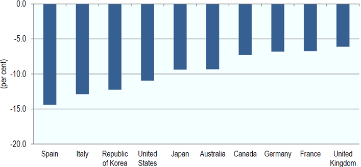
Source: OECD

Source: OECD
Now to the gist of it all – why wealth cannot grow faster than GDP forever and ever. Let’s go back to the November 2021 Absolute Return Letter for a minute, where I introduced the French economist, Thomas Piketty, Professor at Paris School of Economics. Piketty has argued, and that is the argument behind Exhibit 1, that r will continue to grow faster that g, i.e. the ratio of wealth-to-GDP will continue to increase, but that is almost impossible, and here is why.
For the return on capital (r) to exceed the rate of economic growth (g) for longer periods of time, the elasticity of substitution between capital and labour must be greater than one, and I note that, in a recent paper, the elasticity was estimated to be only about 0.3.
For your information, the elasticity of substitution between capital and labour measures “the ease with which one can substitute capital to replace workers, or substitute workers to replace capital, and maintain the same level of output” (source: skaipedia.org). The elasticity of substitution between capital and labour is a key parameter in economics and is critical when seeking to explain the decrease in labour’s share of national income.
Everything would be so much easier if the elasticity of substitution between capital and labour were precisely one. The analysis of many problems would be greatly simplified. However, the elasticity between the two has always been well below one. In other words, wealth cannot continue to grow faster than GDP and, therefore, the inequality gap cannot continue to get bigger and bigger.
How could the theory be proven wrong?
If you read the last few paragraphs once more, you will see that I left the door half-open. Under certain conditions, the elasticity could possibly exceed one and then, suddenly, wealth can continue to grow faster than the underlying economy. What sorts of conditions could lead to that?
For starters, an extreme change of demographics, where the workforce has been virtually extinguished, and few humans work, would most likely lead to an elasticity factor above one. A society run by robots and AI, where humans have become largely obsolete, could probably also do the job.
Having said that, apart from a few extraordinary situations that are not likely to unfold in our lifetime, the elasticity of substitution between capital and labour will almost certainly stay well below one for many years to come. Therefore, mean reversion of wealth-to-GDP will most likely happen, if it hasn’t already started.
Investment implications
If US wealth-to-GDP reverts to its long-term mean value, American household stand to lose over 30% of their wealth. Wealth, both in the US and elsewhere, consists of a mix of property investments, pension savings and investments, whether in listed securities, family-owned business or other. Behind those buckets, three asset classes account for the vast majority, namely equites (both public and private), bonds and property.
My focus today is on US wealth, as that is most out of line (when compared to US GDP), but Europeans and Asians should not consider themselves protected from a US meltdown, even if wealth-to-GDP in other parts of the world is far more modest. US financial markets are so dominant that a US meltdown will almost certainly have a detrimental impact on risk assets all over the world. If US wealth continues to slide, there will be nowhere to hide.
With that caveat, allow me to share my top five investment recommendations in what increasingly looks like a very tricky environment:
1. Be defensive when investing in equities:
a. Reduce the equity beta in your portfolio.
b. Zoom in on value rather than growth stocks.
c. Overweight higher-yielding stocks.
2. Focus on investment themes that will almost certainly unfold regardless of the underlying economic conditions, for example green metals, which stand to benefit from the green transition.
3. Take advantage of the fact that governments all over the world cannot afford for yields to rise too much, i.e. every trick in the book will be utilised to keep borrowing costs down.
4. Stay clear of real estate unless the opportunity is truly unique.
5. Turn your portfolio as uncorrelated as you possibly can. Returns on music royalties are largely uncorrelated. So is uranium (nuclear power plants need uranium whether we are in a recession or not), even if the day-to-day performance of uranium stocks may fluctuate in line with the broader markets.
Take for example 1a above – reduce the equity beta. One obvious way to do that is through an increase in the presence of relative value (RV) trades in the portfolio, so allow me to give you one example. Through our research programme, we have recently concluded that platinum is likely to outperform palladium over the next few years. Both are precious metals and, although platinum is not always a perfect substitute for palladium, the auto industry, which is a major user of both metals in engine exhausts to neutralise harmful emissions, gladly switch from one to the other depending on price. And the price spread is at a tipping point now.
Final few words
By shorting palladium against a long position in platinum, you could establish an RV trade which stands to benefit from a narrowing of the price spread between the two metals. Yet, the equity beta is quite low, i.e. even if a recession is on the horizon (and it is), the RV nature of the trade will most likely protect you from large losses.
Importantly, I should stress that, due to various factors, a long/short position in platinum vs. palladium should not be established 1:1, i.e. with the same notional amount on both sides of the trade. Feel free to contact us, if you want to learn more about this opportunity.
Niels C. Jensen.
12 October 2022
About the Author